Calculated Fields

Overview

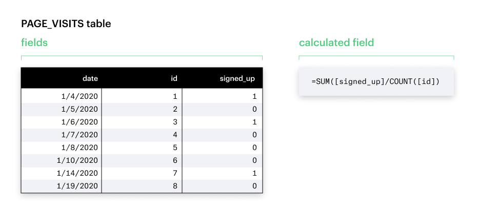
A field is a column in a database table. A calculated field is a field that uses existing database fields and applies additional logic — it allows you to create new data from your existing data.

A calculated field either:

performs some calculation on database fields to create a value that is not directly stored in the database or
selects values in database fields based on some customized criteria

When to Use Calculated Fields

Calculated fields lend to more flexibility and efficiency in your analyses.

Power multiple visual analyses with one query - You can now create multiple calculations on top of one Helix-powered query. Whether you’re exploring your data or answering follow-up questions from your stakeholders, you’ll no longer have to revisit your multiple SQL queries multiple times.
Take full advantage of filtering and drill down features - Previously, some aggregations of pre-aggregated SQL fields led to incorrect results.
Empower non-SQL stakeholders - People who aren’t familiar with SQL but perhaps are familiar with similar tools like Tableau can now answer their own questions.

Some common scenarios for when you’d want to use calculated fields include:

The metrics you need for your analysis are not directly stored in your data warehouse.
You want to transform values for your visualization.
You want to quickly aggregate or filter your data.

Creating a Calculated Field

Navigate to the Mode home page and sign in to your Workspace.
Click the green + to create a new report in the upper righthand corner.
Run a SQL query. (It can be as simple as SELECT * FROM table.)
Create a new chart.
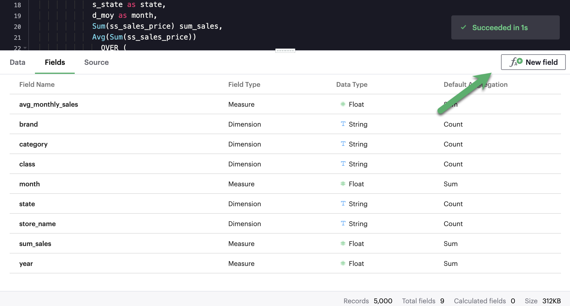
Click the New field button to open the Calculated field formula editor

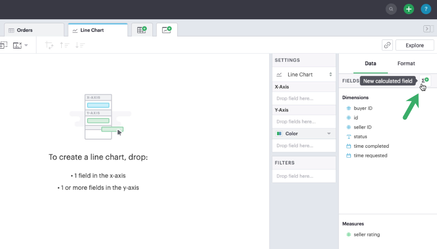
Create calculated field in dataview

From the chart builder, click the New field icon to open the Calculated field formula editor

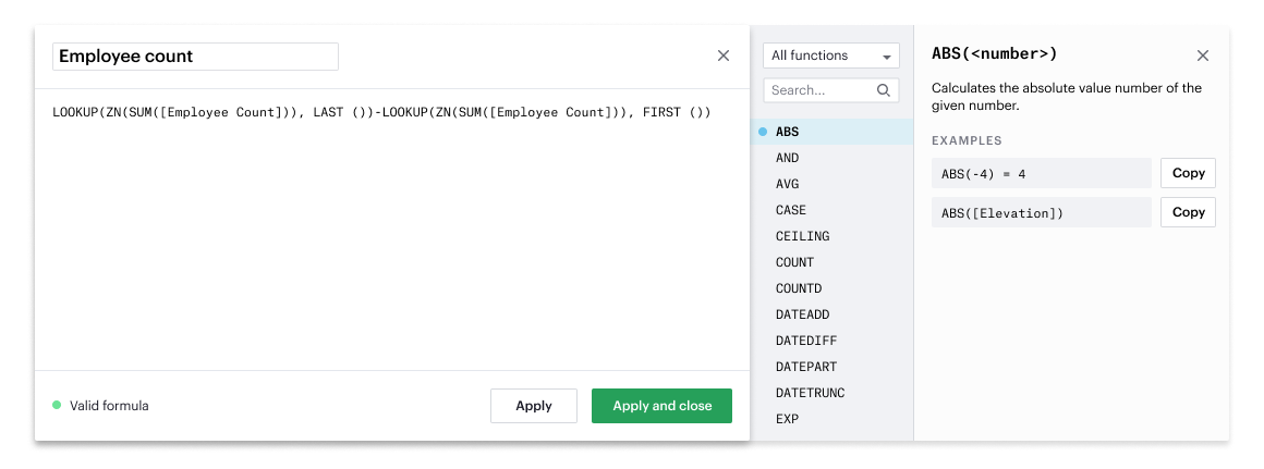
Create calculated field in chart builder

Type in a name and formula for your calculated field. This example uses the formula:

SUM(CASE [Status] WHEN 'CANCELLED' THEN 1 ELSE 0 END)/SUM(1)

This formula checks for whether the order status was cancelled. It will sum up the tally of cancelled orders and divide by the total number of tows to calculate the cancellation rate.

TIP: To see the full list of functions Mode currently supports, open the panel on the righthand side. calculated fields list functions

When you’re done, hit Apply or Done.

Congratulations, you have now created your first calculated field! You should see it in your fields list, with an equal sign (=) next to the data type icon to indicate that it is a calculated field.

Using a Calculated Field

In charts

You can chart your calculated field just as you could a SQL-generated field, by selecting and dragging in the field into your Chart menu.

calculated fields in charts

In filters

You can also filter your calculated field just as you could a SQL-generated field.

Calculated Fields in Filters

Calculated Field Best Practices

Calculation building blocks

These are the four basic components that make up any calculated field:

Fields - columns from your data source, can be either a Dimension or a Measure.
Operators - symbols that denote a certain operation, like + and - .
Functions - transforms the given input to an expected output, like COUNT() and SUM().
Literal expressions - constant values that are represented as is. This includes numbers (1), strings ("This is a string"), dates (#2020-06-01#), booleans (true), and null.

Additionally, calculated fields can also contain:

Parameters - fixed values that functions expect as input, such as 'week' in DATEPART() .
Comments - notes or commentary about the calculation that will not be included in the computation. Comments in calculated fields are always marked by a prepended //.

Field properties

Property	Description	In Mode
Dimension	Fields that are used to slice and describe data records (e.g. names, dates, )
Measure	Typically the values corresponding to the dimension that will be aggregated (e.g. sum, count, average)
Discrete	Values in the dataset are distinct and separate. These fields are indicated in Mode with blue icons.
Continuous	Values in the dataset can take on any value within a finite or infinite range. These fields are indicated in Mode with green icons.

Available Operators

Precedence	Symbol	Name	Description	Example
1	- (negate)	Negate	Negates the numeric input	`-1`
2	*	Multiplication	Multiplies two numeric types together	`5 * 4 = 20`
3	/	Division	Divides the first numeric input by the second numeric input	`20 / 4 = 5`
4	+	Addition	Adds two numeric types together	`2 + 2 = 4`
4	- (subtract)	Subtraction	Subtracts two numeric types	`10 - 8 = 2`
5	=	Equal to	Compares two numbers, dates, or strings and returns either TRUE, FALSE, or NULL.	`5 + 5 == 10`
5	>	Greater than	Compares two numbers, dates, or strings and returns either TRUE, FALSE, or NULL.	`6 > 5 = TRUE`
5	<	Less than	Compares two numbers, dates, or strings and returns either TRUE, FALSE, or NULL.	`6 < 5 = False`
5	>=	Greater than or equal to	Compares two numbers, dates, or strings and returns either TRUE, FALSE, or NULL.	`5 >= 5 = TRUE`
5	<=	Less than or equal to	Compares two numbers, dates, or strings and returns either TRUE, FALSE, or NULL.	`4 <= 5 = TRUE`
5	<>	Not equal to	Compares two numbers, dates, or strings and returns either TRUE, FALSE, or NULL.	`5 != 'five' = TRUE`
6	NOT	Not	Negates the boolean or expression	`NOT FALSE = TRUE`
7	AND	And	An expression or boolean must evaluate to TRUE on both sides of the AND	`TRUE AND FALSE = FALSE`
8	OR	Or	An expression or boolean must evaluate to TRUE on at least one side of the OR	`TRUE OR FALSE = TRUE`

Precedence dictates the order in which operators will be evaluated in a formula. Parentheses can be used to change the order of precedence.

Available functions

Number

Function	Description	Examples
`ABS(<number>)`	Returns the absolute number of the given number.	`ABS(-4) = 4` `ABS([Elevation])`
`CEILING(<number>)`	Rounds a number to the nearest integer of greater than or equal value.	`CEILING(3.14159) = 4` `CEILING([Order Price])`
`EXP(<number>)`	Returns e raised to the power of the given number, where e is the Euler’s constant 2.718...	`EXP(2) = e^2` `EXP([Order Quantity])`
`FLOOR(<number>)`	Rounds a number to the nearest integer of less than or equal value.	`FLOOR(3.14159) = 3` `FLOOR([Order Price])`
`LOG10(<number>)`	Returns the base 10 logarithm of a number.	`LOG10(100) = 2` `LOG10([Order Quantity])`
`LN(<number>)`	Returns the natural logarithm of a number, where the base is Euler’s constant e.	`LN(EXP(2)) = 2` `LN([Order Quantity])`
`MOD(<number>,` `<number>)`	Divides the first number by the second number and returns their remainder.	`MOD(11, 2) = 1` `MOD([Order Quantity], 100)`
`POWER(<base number>,` `<exponent number>)`	Returns the base raised to the inputted exponent power.	`POWER(2, 3) = 8` `POWER([Order Quantity],` `[Price])`
`ROUND(<number>, <number>)`	Returns the number rounded to the nearest specified decimal place.	`ROUND(3.14159, 4) = 3.1416` `ROUND(AVG([Profit]), 2)`
`SQRT(<number>)`	Returns the square root of the given number.	`SQRT(9) = 3` `SQRT([Order Quantity])`
`TRUNC(<number>,` `<number>)`	Returns the number cut off to the specified decimal place.	`TRUNC(3.14159, 2) = 3.14` `TRUNC(AVG([Profit]), 2)`
`ZN(<expression>)`	Returns the given expression if not `NULL`, otherwise returns 0.	`ZN(1, NULL, 1) = 1, 0, 1` `ZN[Order Quantity])`

String

Function	Description	Examples
`CONTAINS(<string>,` `<substring>)`	Returns TRUE if the substring is within the string, otherwise returns FALSE.	`CONTAINS('Hello world!', 'lo w') = True` `CONTAINS('Hello world!' 'hello') = False` `CONTAINS([status], 'error')`
`FIND(<string>, <subString>, [<start>])`	Returns the index position of substring in string or 0 if the substring isn't found. First character of the string is at position 1. Start is an optional argument to define from where to start the search.	`FIND('hello', 'l', 1)` `FIND([Address], 'Unit')`
`LEFT(<string>, <count>)`	Extract the left most count characters	`LEFT('hello', 2)` `LEFT([Address], 3)`
`LOWER(<string>)`	Returns string with all characters lowercased.	`LOWER('Hello World!')` `LOWER([status])`
`LTRIM(<string>)`	Removes any spaces from the left side of the string.	`LTRIM(' Hello World!')` `LTRIM([status])`
`PLUCK(<string>, <delimiter>, <tokenIndex>)`	Splits the string along the separator/delimiter, returning the string at the corresponding token index.	`PLUCK('John Smith', ' ', 2)` `PLUCK([address], '-', 2)`
`REPLACE(<string>, <searchString>, <replaceString>)`	Replaces all occurrences of the search string with the replace string.	`REPLACE('hello', 'l', '-')` `REPLACE([Address]'Ceylon', 'Sri Lanka')`
`RIGHT(<string>, <count>)`	Extract the right most count characters	`RIGHT('hello', 2)` `RIGHT([Address], 3)`
`RTRIM(<string>)`	Removes any spaces from the right side of the string.	`RTRIM('Hello World! ')` `RTRIM([status])`
`SUBSTR(<string>, <start>, [<length>])`	Returns the substring beginning at start. Note that a start value of 1 refers to the first character of the string. If length is provided, the returned substring will include that number of characters at most	`SUBSTR('hello', 2, 2)` `SUBSTR([Address], 4)`
`TRIM(<string>)`	Removes any spaces from either side of the string.	`TRIM(' Hello World ')` `TRIM([status])`
`UPPER(<string>)`	Returns string with all characters uppercased.	`UPPER('Hello World!')` `UPPER([status])`

Datetime

Function	Description	Examples
`DATEADD(<datepart>,` `<interval>,` `<datetime>)`	Adds the specified datepart to the given datetime, where	`DATEADD('week', 4, TODAY()) = #2020-06-29#` `DATEADD('quarter', -1, [Date])`
`DATEDIFF(<datepart>,` `<datetime1>,` `<datetime2>)`	Finds the difference between the two datetimes expressed in units of the given datepart. In the examples on the right, the first expression returns 0 because the two dates are in the same month. The second expression returns 1 because the second date is in a new month, even though the two dates are not 30 days apart.	`DATEDIFF('month', #2020-06-08#, #2020-06-25#) = 0` `DATEDIFF('month', #2020-06-29#, #2020-07-03#) = 1`
`DATEPART(<datepart>,` `<datetime>)`	Returns the specified part of the given datetime expression as a number. The returned number may change based on the day specified as start of the week or start of year. If not specified, the default for start of week is Sunday and the default start of year is January. Start of year option only applies to quarter and year. Please note that to specify the start of year, the start of week needs to be specified too.	`DATEPART('day', #2020-06-01#) = 1` `DATEPART('month', #2020-06-01#) = 6` `DATEPART('year', #2020-06-01#) = 2020` `DATEPART('WEEK', #2023-12-31#, 'MONDAY') = 52` `/Default is SUNDAY/` `DATEPART('WEEK', #2023-12-31#) = 1` `DATEPART('quarter', #2023-12-31#, 'SUNDAY',’AUGUST’) = 2` `/Default is JANUARY/` `DATEPART('quarter', #2023-12-31#) = 4`
`DATETRUNC(<datepart>,` `<datetime>)`	Returns a date value equal to the given datetime expression truncated to the specified precision. The returned date value may change based on the day specified as start of the week or start of year. If not specified, the default for start of week is Sunday and the default start of year is January. Start of year option only applies to quarter and year. Please note that to specify the start of year, the start of week needs to be specified too.	`DATETRUNC('month', #2020-06-29#) = #2020-06-01#` `DATETRUNC('quarter', [Order Date])` `DATETRUNC('WEEK', #2023-12-31#, 'MONDAY') = #2023-12-25#` `/Default is SUNDAY/` `DATETRUNC('WEEK', #2023-12-31#) = #2023-12-31#` `DATETRUNC(('quarter', #2023-12-31#, 'SUNDAY',’AUGUST’) = 2023-11-01` `/Default is JANUARY/` `DATETRUNC('quarter', #2023-12-31#) = 2023-10-01`
`NOW()`	Returns the current datetime.	`NOW() = #2020-06-01 9:00:00 AM#`
`TODAY()`	Returns the current date.	`TODAY() = #2020-06-01#`

Possible <datepart> values include:

second
minute
hour
day
week
weekday
month
dayofyear
quarter
year

Week Start Day customization

Week Start Day option in the context menu for date fields can be used to customize the week start day to be any day of the week. The default is Sunday. This selection will also be reflected in the +/- granularity controls on the chart.

Week Start Day customization in Quick Charts

Week Start Day Quick Charts

Week Start Day customization in Visual Explorer

Week Start Day Visual Explorer

Year Start customization

Year Start option in the context menu for date fields in Quick Charts and Visual Explorer can be used to customize the start of year to be any month of the year. The default is January. This selection will also be reflected in the +/- granularity controls on the chart. The year start can be adjusted in visualization filters to match the chart by using the settings gear icon in the filter modal.

Year start customization in Quick Charts and Visual Explorer

Type Conversion

Function	Description	Examples
`DATE(<expression>)`	Convert expression to YYYY-MM-DD date format. Returns `NULL` if expression cannot be converted to datetime.	`DATE(1672542245050) // #2023-01-01#` `DATE("2023-02-01T05:30:15.050Z") // #2023-02-01#` `DATE(#2023-02-01T05:30:15.050Z#) // #2023-02-01#`
`DATETIME(<expression>)`	Convert expression to YYYY-MM-DD HH:MM:SS format. Returns `NULL` if expression cannot be converted to datetime	`DATETIME(1672542245050) // #2023-01-01 03:04:05#` `DATETIME("2023-02-01T05:30:15.050Z") // #2023-02-01 05:30:15#` `DATETIME(#2023-02-01#) // #2023-02-01 00:00:00#`
`INT(<expression>)`	Convert the given expression to an integer. The results are rounded towards zero.	`INT(10.5) //10` `INT("10.5") //10` `INT("-10.5") //-10` `INT(true) //1` `INT(#2023-02-01T05:30:15.050Z#) //1675229415050`
`FLOAT(<expression>)`	Convert the given expression to a floating point number.	`FLOAT(10.5) //10.5` `FLOAT("10.5") //10.5` `FLOAT(true) //1` `FLOAT(#2023-02-01T05:30:15.050Z#) //1675229415050`

Logical

Function	Description	Examples
`<expression1> AND <expression2>`	Returns TRUE if and only if both expressions are true.	`2 > 1 AND 2 > 3 = False` `[Order Date] >= TODAY()` `AND [Order Amount] > 1`
`CASE <expression>` `WHEN <value1> THEN <return1>` `[WHEN <value2> THEN <return2>` `...]` `ELSE <default return> END`	Performs a series of logical tests for equality and returns the value of the test that first evaluated to true.	`CASE [Status]` `WHEN 'Completed' THEN 1` `WHEN 'Cancelled' THEN 0` `ELSE NULL END`
`IF <expression> THEN <return1>` `[ELSEIF <expression2> THEN` `<return2>` `...]` `ELSE <default return> END`	Performs a series of logical tests, not necessarily always for equality, and returns the value of the test that first evaluated to true.	`IF [Profit] > 0 THEN 'Profitable'` `ELSEIF [Profit] = 0 THEN 'Breakeven'` `ELSE 'Nonprofitable' END`
`<expression1> OR <expression2>`	Returns TRUE as long as one of the expressions is true.	`2 > 1 OR 2 > 3 = True` `[Order Amount] >= 5 OR [Price] >= 50`
`ISNULL(<expression>)`	Returns TRUE if `<expression>` is `NULL`	`ISNULL(NULL) = TRUE` `ISNULL([Order Amount])`
`IFNULL(<expression>, <altExpression>)`	Returns `<expression>` if it is not `NULL`, otherwise returns `<altExpression>`. If both inputs are `NULL` then `NULL` is returned.	`IFNULL(10, 5) = 10` `IFNULL(NULL, 1) = 1`

Aggregate

Function	Description	Example
`AVG(<expression>)`	Averages the values of items in a group, not including `NULL` values.	`AVG(1, 2, 3, 10) = 4` `AVG([Order Amount])`
`COUNT(<expression>)`	Counts the total number of items in a group, not including `NULL` values.	`COUNT([1, 2, 2, 4]) = 4` `COUNT([Order Id])`
`COUNTD(<expression>)`	Counts the total number of distinct items in a group, not including `NULL` values.	`COUNTD([1, 2, 2, 4]) = 3` `COUNTD([Order Id])`
`KURT(<expression>)`	Returns the excess kurtosis of all input values.	`KURT([Order Quantity])`
`MAX(<expression>)`	Computes the item in the group with the largest numeric value.	`MAX([1, 2, 2, 4]) = 4` `MAX([Order Amount])`
`MEDIAN(<expression>)`	Computes the median of an expression, which is the value that the values in the expression are below 50% of the time.	`MEDIAN([1, 2, 3, 4, 5]) = 3` `MEDIAN([1, 2, 3, 10]) = 2.5` `MEDIAN([Order Amount])`
`MIN(<expression>)`	Computes the item in the group with the smallest numeric value.	`MIN([1, 2, 2, 4]) = 1` `MIN([Order Amount])`
`MODE(<expression>)`	Returns the most frequent value for the values within x. `NULL` values are ignored.	`MODE([Order Quantity])`
`PERCENTILE_1(<expression>)`	Computes the 1st percentile within an expression, which is the value that the values in the expression are below 1% of the time.	`PERCENTILE_1([1, 2, 3, 4, 5]) = 1.04` `PERCENTILE_1([Order Amount])`
`PERCENTILE_5(<expression>)`	Computes the 5th percentile within an expression, which is the value that the values in the expression are below 5% of the time.	`PERCENTILE_5([1, 2, 3, 4, 5]) = 1.2` `PERCENTILE_5([Order Amount])`
`PERCENTILE_25(<expression>)`	Computes the 25th percentile within an expression, which is the value that the values in the expression are below 25% of the time.	`PERCENTILE_25([1, 2, 3, 4, 5]) = 2` `PERCENTILE_25([Order Amount])`
`PERCENTILE_75(<expression>)`	Computes the 75th percentile within an expression, which is the value that the values in the expression are below 75% of the time.	`PERCENTILE_75([1, 2, 3, 4, 5]) = 4` `PERCENTILE([Order Amount])`
`PERCENTILE_95(<expression>)`	Computes the 95th percentile within an expression, which is the value that the values in the expression are below 95% of the time.	`PERCENTILE_95([1, 2, 3, 4, 5]) = 4.8` `PERCENTILE_95([Order Amount])`
`PERCENTILE_99(<expression>)`	Computes the 99th percentile within an expression, which is the value that the values in the expression are below 99% of the time.	`PERCENTILE_99([1, 2, 3, 4, 5]) = 4.96` `PERCENTILE_99([Order Amount])`
`SKEW(<expression>)`	Returns the skewness of all input values.	`SKEW([Order Quantity])`
`STDEV(<expression>)`	Returns the standard deviation of all values in the given expression based on a sample of the population.	`STDEV([Order Quantity])`
`STDEVP(<expression>)`	Returns the standard deviation of all values in the given expression based on the entire population	`STDEVP([Order Quantity]`
`SUM(<expression>)`	Sums the total number of items in a group, not including `NULL` values.	`SUM([1, 2, 2, 4]) = 9` `SUM([Order Amount])`
`VAR(<expression>)`	Returns the variance of all values in the given expression based on a sample of the population.	`VAR([Order Quantity])`
`VARP(<expression>)`	Returns the variance of all values in the given expression based on the entire population	`VARP([Order Quantity])`

Analytical

Function	Description	Examples
`FIRST()`	Returns the number of rows from the current row to the first row of the partition.	`(Current row index is 2 of 5)` `FIRST() = -1`
`INDEX()`	Returns the index of the current row in the partition.	`(Current row index is 2 of 5)` `INDEX() = 2`
`LAST()`	Returns the number of rows from the current row to the last row of the partition.	`(Current row index is 2 of 5)` `LAST() = 3`
`LOOKUP(<expression>, [<offset>])`	Returns the value of the expression in a target row and can be specified as a relative offset number from the current row.	`LOOKUP(SUM([Order Quantity]), INDEX()) = SUM(Order Quantity) in the current row of the partition`
`NTILE(<expression>, <number>, [<order>])`	Distributes the rows in an ordered partition into the specified (integer) number of groups. The groups are numbered, starting at one. For each row, NTILE returns the number of the group to which the row belongs. The default order is descending.	`NTILE(SUM([Order Amount]), 4, "ASC")`
`RANK(<expression>, [<order>])`	Returns the rank of each row within the partition of a result set. The rank of a row is one plus the number of ranks that come before the row in question. The default order is descending.	`RANK(SUM([Order Amount]), "ASC")`
`RANK_DENSE(<expression>, [<order>])`	Returns the rank of each row within a result set partition, with no gaps in the ranking values. The rank of a specific row is one plus the number of distinct rank values that come before that specific row. The default order is descending.	`RANK_DENSE(SUM([Order Amount]), "DESC")`
`RUNNING_AVG(<expression>)`	Returns the running average of the given expression, from the first row in the partition to the current row. The given expression must be either an aggregate or a constant.	`RUNNING_AVG(SUM([Order Amount])`
`RUNNING_COUNT(<expression>)`	Returns the running count of the given aggregate expression, from the first row in the partition to the current row. The given expression must be either an aggregate or a constant.	`RUNNING_COUNT(COUNT([Order Id])`
`RUNNING_SUM(<expression>)`	Returns the running sum of the given aggregate expression, from the first row in the partition to the current row. The given expression must be either an aggregate or a constant.	`RUNNING_SUM(SUM([Order Amount])`
`TOTAL(<expression>)`	Returns the total for the given expression, calculated using all rows within that partition.	`TOTAL(SUM([order_amount])) = the total sum of the order amount for all rows within the partition.`
`WINDOW_AVG(<expression>,` `[<start>, <end>])`	Returns the average of the given expression within the window. The window is defined by means of offsets from the current row. The given expression must be either an aggregate or a constant. `<start>` and `<end>` are optional integer parameters that define the partition. They are indices based on the current reference point If the start and end are omitted, the entire partition is used. `FIRST()+n` and `LAST()-n` are can be used as offsets from the first or last row in the partition
`WINDOW_COUNT(<expression>,` `[<start>, <end>])`	Returns the count of the given expression within the window. The window is defined by means of offsets from the current row. The given expression must be either an aggregate or a constant.`<start>` and `<end>` are optional integer parameters that define the partition. They are indices based on the current reference point (see picture below) If the start and end are omitted, the entire partition is used. FIRST()+n and LAST()-n are can be used as offsets from the first or last row in the partition.
`WINDOW_SUM(<expression>,` `[<start>, <end>])`	Returns the sum of the given expression within the window. The window is defined by means of offsets from the current row. The given expression must be either an aggregate or a constant. `<start>` and `<end>` are optional integer parameters that define the partition. They are indices based on the current reference point (see picture below) If the start and end are omitted, the entire partition is used. FIRST()+n and LAST()-n are can be used as offsets from the first or last row in the partition.

💡 For calculated field window functions, it'll be helpful to understand how window partitions are defined.

SQL allows you to perform aggregations in different levels of the view using window functions, generally written as OVER (PARTITION BY column). Window functions also exist in calculated fields, though the way you define window partitions is different.

Instead of specifying the partition directly in the formula code, you'd drag and drop the field into your chart axis along with your window calculated field. The system will automatically re-calculate the values depending on your dimension.
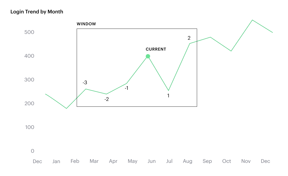
For moving windows, you'd specify a <start> and <end> relative to the current row
- In general, -n refers to the nth row before the current row, and n refers to the nth row after the current row.
- You can also crate offsets based on the first or last rows in the expression, using FIRST()+n and LAST()-n.
  - FIRST() always returns -1 for the second row, -2 for the third row, etc.
  - LAST() always returns 1 for the second-to-last row, 2 for the third-to-last row, etc.

The corresponding formula for this window sum would be WINDOW_SUM(SUM([field]), -3, 2).

Calculated Field Component Types

Unlike your SQL results, which are always constants, calculated fields have different computation levels:

Order	Type	Description	Examples
1	Constant	A fixed value.	`1` `TRUE`
2	Scalar	Values are mapped to a single result in a one-to-one manner.	`ABS()` `DATEDIFF()`
3	Aggregate	Values of multiple rows are grouped together as the input to form a single value of more significant meaning.	`COUNT()` `SUM()`
4	Analytical	Computes aggregate values over a group of rows.	`LOOKUP()` `RUNNING_SUM()`

Component Operations

You can combine various component types in operation.

Example:

1 + [column] will add 1 to every row in your column. The result of that operation will take the greatest order of the combined data types — constant + scalar returns a scalar result.
1 + SUM([column])

However, there are limitations to what calculated fields you can use in functions.

Non-examples:

Aggregating an aggregate - SUM(COUNT([column])) ❌
Mixing aggregate and non-aggregate values in certain functions - DATEDIFF('day', created_at, MAX(updated_at)) ❌
Using scalar values in an analytical function - RUNNING_COUNT([id]) ❌

FAQs

Q: How do you get the running percentage total of a field?

We do have some ways of utilizing analytic functions within our calculated fields to calculate percent over total. Check out this blog on Analytic Functions and how to use them in Mode.

Q: How to do a CASE statement where the condition is a comparison (e.g. <=)?

You use CASE statements for direct equality against one field. For example:

CASE [status] 
WHEN 'Completed' THEN 1 
WHEN 'Cancelled' THEN 0 
ELSE NULL END

If you wish to compare multiple fields or use comparisons, then you’d use an IF statement. For example:

IF [revenue] > 0 OR [cost] < 0 THEN 'Profitable'
ELSEIF [revenue] = 0 OR [cost] = 0 THEN 'Neutral'
ELSE 'Unprofitable'
END

Q: Are special characters allowed in the calculated field name?

We currently do not allow brackets like [ and ] in the calculated field name. This is for parsing and usability reasons, because you can reference calculated fields by their names in other calculated field formulas.

Troubleshooting

1. Why am I getting a 'Cannot combine aggregate and non-aggregate fields' error?

You cannot directly combine and/or compare aggregate and non-aggregate fields because they are different component types.

Let’s say your non-aggregate field contains the data [1, 2, 3, 4, 5]. It has a cardinality of 5.
An aggregate calculated field, such as SUM([field]) yields the result 15. It has a cardinality of 1.

2. My Calculated Field is not saving

A Calculated Field will not be saved if it exceeds the maximum number of characters (1024). Please ensure that your Calculated Field does not exceed this limit in order to save it successfully.

If the issue is not the above, please don't hesitate to reach out to our Support team for further assistance.

Was this article helpful?

Get a firsthand look at Mode's key features & workflows

Mode Help