Back in August, we released Calculated Fields, a feature that allows analysts to work more quickly by performing post-SQL analysis. Now, we’re excited to bring you a new set of formulas within Calculated Fields: Analytic Functions. Analytic functions make Calculated Fields even more powerful by allowing you to calculate metrics based on specified partitions of your data.

What are analytic functions?

Analytic functions allow you to perform computations across a set of table rows that are somehow related to the current row. They are calculated based on what is currently in your visualization and do not consider any values that are filtered out of the visualization.

There are three types of analytic functions:

1. Analytic aggregation functions

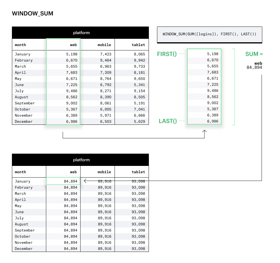
RUNNING_AVG, RUNNING_COUNT, RUNNING_SUM
WINDOW_AVG, WINDOW_COUNT, WINDOW_SUM

2. Analytic navigation functions

FIRST
LAST
LOOKUP

3. Analytic number functions

INDEX

Window functions are a powerful analytic aggregation function. They perform calculations across a set of rows in your dataset that are related to the current row. However, window functions do not cause the rows to become grouped into a single output like aggregate functions do (e.g., SUM). Instead, the returned output still contains the individual rows.

In SQL, you may specify the specific rows to use in a window function like so:

SELECT 
    SUM(columnA) OVER (ORDER BY columnB
    ROWS BETWEEN 3 PRECEDING AND CURRENT ROW) AS current_and_prev3
FROM my_table

Similarly, in Calculated Fields, you’d define windows by how many steps a datapoint is from your current index.

window-animation

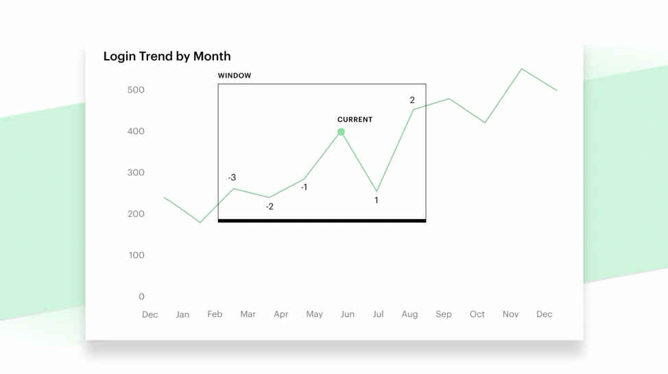
If a window is not specified or the range is set as the first and last indices, the system will calculate over the entire frame, like so:

window sum

How to use analytical functions

To get started, let’s walk through a few specific examples of analytic functions and how to use them.

Let’s say that you are tasked with building your company’s sales metrics. Instead of writing multiple custom SQL queries, you decide to leverage Mode’s new Calculated Fields to build these metrics on top of your raw dataset that will recalculate based on your visualization configurations.

You have the following fields in your sales dataset:

id
timestamp
amount

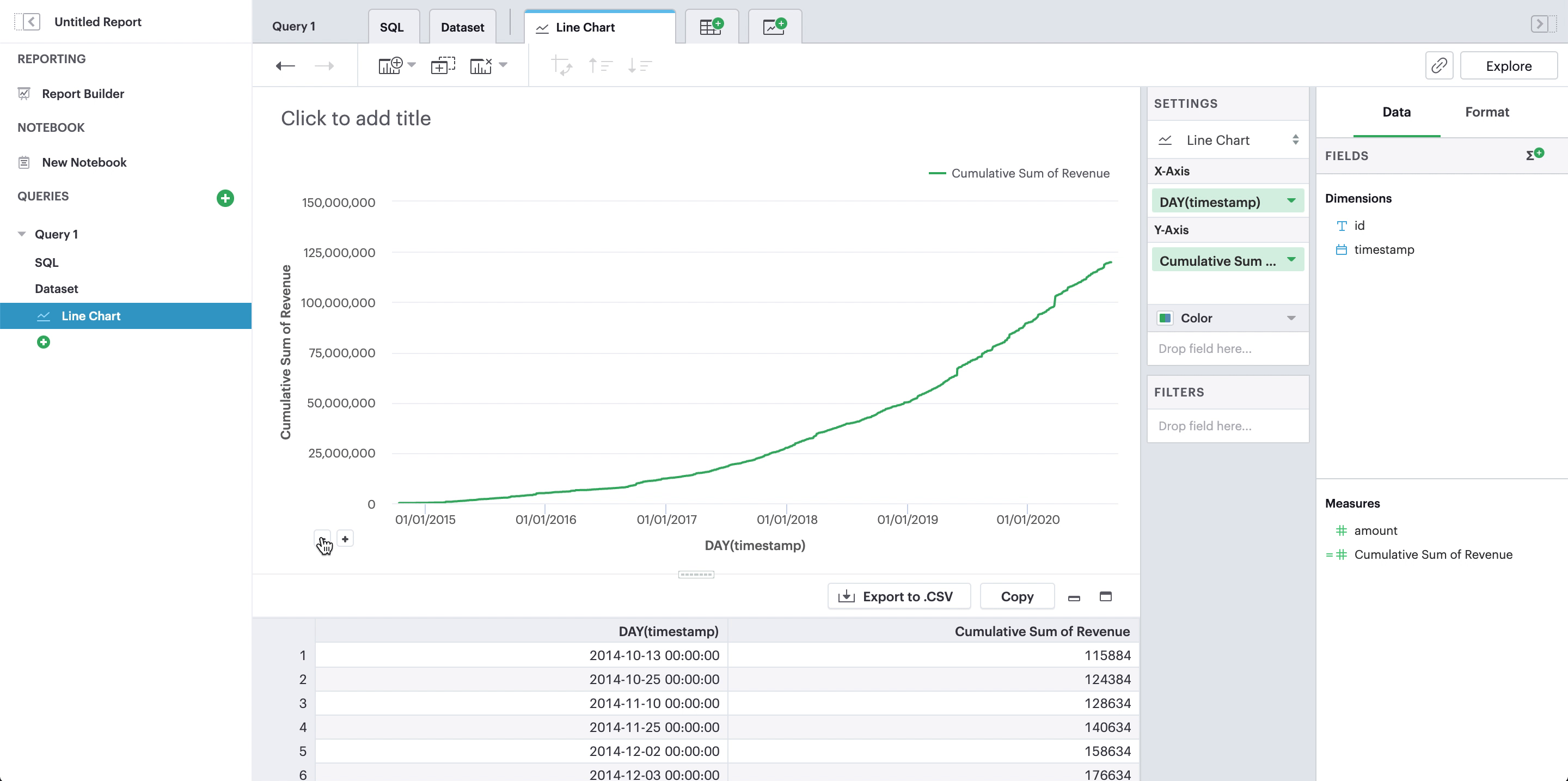
1. Cumulative sum of revenue

We’re interested in a cumulative sum of all the revenue we’ve generated in a given time frame. We can now calculate this in Calculated Fields, using the RUNNING_SUM analytic function.

Create a calculated field using this formula:

RUNNING_SUM(SUM([amount]))

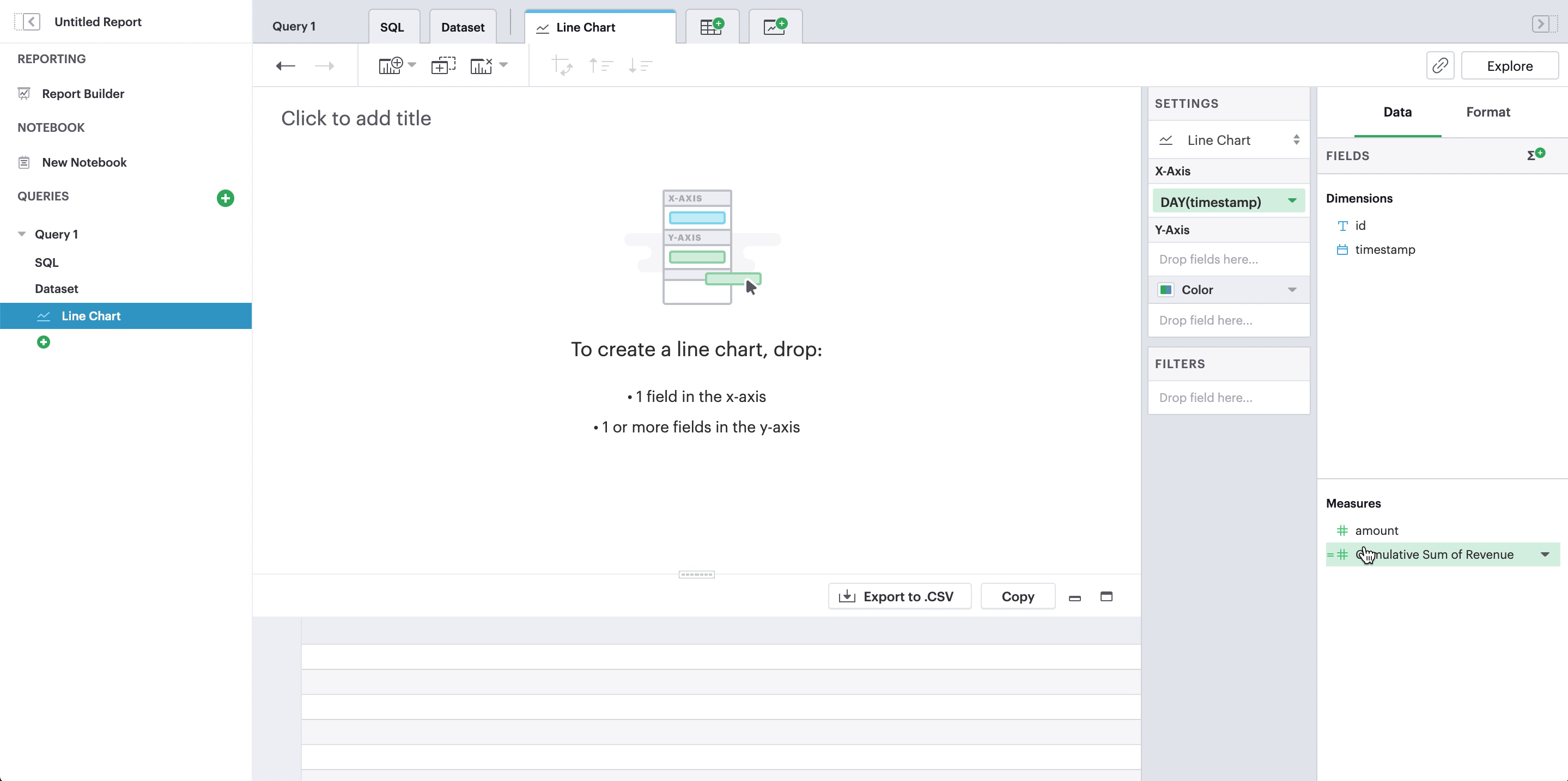
and drag our new field to the y-axis of our line chart.

cumulative sum

For our x-axis, we can add a field of any time granularity or even change it later—our new calculated field will recalculate on the fly! granularities

2. Rolling 7-day revenue average

We’re also interested in understanding what our average daily revenue is. Because our revenue can fluctuate day-by-day, we may look at our revenue averages through a rolling period.

For a 7-day window, we can create a calculated field like so:

WINDOW_AVG(SUM([amount]), -6, 0)

and add it to our y-axis. This function calculates the average of the total amount between the previous 6 rows and the current row.

For our x-axis, this time we want to explicitly use day as the time granularity because we want a 7-day window.

This formula calculates the total amount per day, SUM([amount]), and then finds the average of that date (indexed 0) and the 6 days before that date.

3. Percent of total revenue

Analytic functions also allow us to calculated percentages based on the total.

Window functions, when there is no window specified, will calculate over the entire dataset. We can use this as the denominator in our percentage calculation:

SUM([amount])/WINDOW_SUM(SUM([amount]))

And just like before, we can use any time granularity on the x-axis and update them at any time because our calculated field will be recalculated every time.

4. Year over year change of weekly revenue

We’re getting fancy now. We can use the LOOKUP analytic function to look up previous data points based on the current index. This allows us to reference data points that aren’t the current index and use that in calculations with the current index.

To calculate the percent change of this year’s weekly revenue from last year’s weekly revenue, we can use the LOOKUP function to look back 52 weeks:

LOOKUP(SUM([amount]), -52)

Then, we can use our newly created calculated field to calculate the percent change compared to this week’s revenue:

SUM([amount])/[last_year_amount] - 1

Because we’re looking back specifically 52 rows, we want to use **week** on the x-axis.

Try it yourself!

You can find the complete list of analytic functions we currently support, along with documentation of each function, in our functions library.

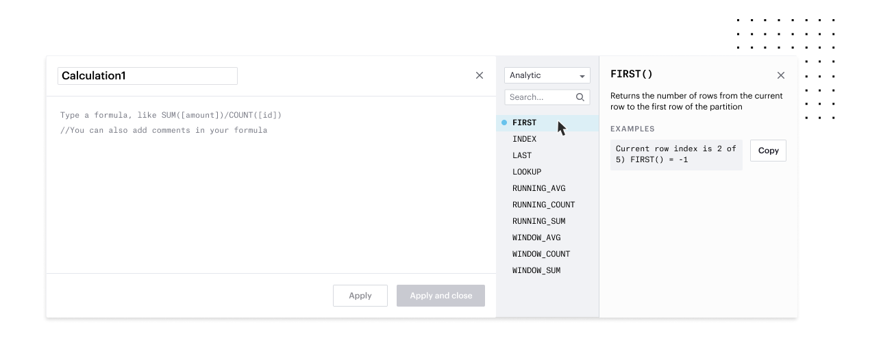try-it-today Pictured: You can view the list of functions we support and filter for specific function types, such as analytic functions, in our functions library.