Forecasting in R with Prophet
Forecasting is often considered a natural progression from reporting. Reporting helps us answer what happened? Forecasting helps answer the next logical question: what will happen?
Historically, high-quality forecasts have been very challenging to produce. This resulted in a severe shortage of analysts who could deliver forecasts with the level of accuracy required to drive business decisions. To alleviate this supply gap and to make scalable forecasting dramatically easier, the Core Data Science team at Facebook created Prophet, a forecasting library for Python and R, which they open-sourced in 2017.
The intent behind Prophet is to “make it easier for experts and non-experts to make high-quality forecasts that keep up with demand.” Prophet is able to produce reliable and robust forecasts (often performing better than other common forecasting techniques) with very little manual effort while allowing for the application of domain knowledge via easily-interpretable parameters.
In this recipe, you'll learn how to use Prophet (in R) to solve a common problem: forecasting a company's daily orders for the next year. This lightweight example should serve as a great way to get started with Prophet, and will hopefully spark some inspiration to dive even deeper into the library's vast functionality.
This recipe is broken down into four main sections:
You can find implementations of all of the steps outlined below in this example Mode report.
Data Preparation & Exploration
Prophet works best with daily periodicity data with at least one year of historical data. It's possible to use Prophet to forecast using sub-daily or monthly data, but for the purposes of this recipe, we'll use the recommended daily periodicity. We will use SQL to wrangle the data we’d like to forecast at a daily periodicity:
`select
``  date,
  value
from modeanalytics.daily_orders
order by date`
NOTE: While Prophet is relatively robust to missing data, it’s important to ensure that your time series is not missing a significant number of observations. If your time series is missing a large number of observations, consider using a resampling technique or forecasting your data at a lower frequency (e.g. making monthly forecasts using monthly observations)
Now that we have our data at a daily periodicity, we can pipe our SQL query result set into an R dataframe object in the R notebook. First, rename your SQL query to Daily Orders. Then, inside the R notebook, we can use the following statement to pipe our query result set into a dataframe df:
df <- datasets[["Daily Orders"]]
To get a quick sense of how many observations your dataframe contains, you can run the following statement:
# Retreive dimension of object
dim(df)
Prophet always expects two columns in the input DataFrame: ds and y, containing the date and numeric values respectively. To check the types of the columns in your DataFrame, you can run the following statement in the R notebook:
# Inspect variables
str(df)
In this example, you'll need to do some manual class conversion:
# Parse date column
df <- mutate (
df,
date = ymd_hms(date) # parse date column using lubridate ymd_hms function
)
Once you have confirmed that the columns in your dataframe are the correct classes, you can create a new column ds in your dataframe that is an exact copy of the date column, and a new column y that is an exact copy of the value column:
df <- mutate (
df,
ds = date,  # Create new ds column from date using mutate
y = value   # Create new y column from value using mutate
)
You can then repurpose the date column to be used as the index of the dataframe:
# # Repurpose date column to be used as dataframe index
df <- column_to_rownames(df, var = "date")
Now that you have your data prepped to be used with Prophet, it’s good practice to plot it and inspect what the data looks like before feeding it into Prophet. Using our example data, we can use ggplot2 to create the following visualization:
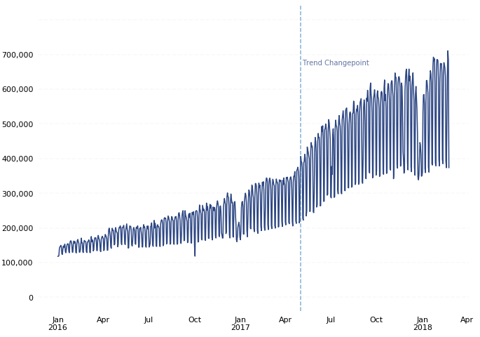
There are a few things to notice about this plot:
- There is a noticeable change in trend trajectory around May 2017. By default, Prophet automatically detects these kinds of “trend changepoints” and allows the trend to adapt appropriately. Prophet also allows finer-grained control over the identification of these trend changepoints.
- There is noticeable weekly and yearly seasonality. Prophet will automatically fit weekly and yearly seasonalities if the time series is more than two cycles long.
- The mean and variance of our observations increase over time. Prophet natively models the increase in mean of the data over time, but we should take additional steps to normalize as much variance as possible to achieve the most accurate forecasting results. We can do this by applying a power transform to our data.
Box-Cox Transform
Often in forecasting, you'll explicitly choose a specific type of power transform to apply to the data to remove noise before feeding the data into a forecasting model (e.g. a log transform or square root transform, amongst others). However, it can sometimes be difficult to determine which type of power transform is appropriate for your data. This is where the Box-Cox Transform comes in.
Box-Cox Transforms are data transformations that evaluate a set of lambda coefficients (λ) and selects the value that achieves the best approximation of normality.
The R forecast library provides a built-in Box-Cox Transform function, called BoxCox(). The BoxCox() function has two required inputs: a numeric vector or time series of class ts and and a lambda coefficient transformation parameter. To determine the lambda coefficient to use in the Box-Cox transformation, you can use the built-in BoxCox.lambda() function, which automatically selects the optimal lambda coefficient for the transformation.
For our example, we will let the [BoxCox.lambda()](https://www.rdocumentation.org/packages/forecast/versions/8.1/topics/BoxCox.lambda) function determine the optimal λ to use for the transformation, and will then use that value in the BoxCox() function:
# The BoxCox.lambda() function will choose a value of lambda
lam = BoxCox.lambda(df$value, method = "loglik")
df$y = BoxCox(df$value, lam)
df.m <- melt(df, measure.vars=c("value", "y"))
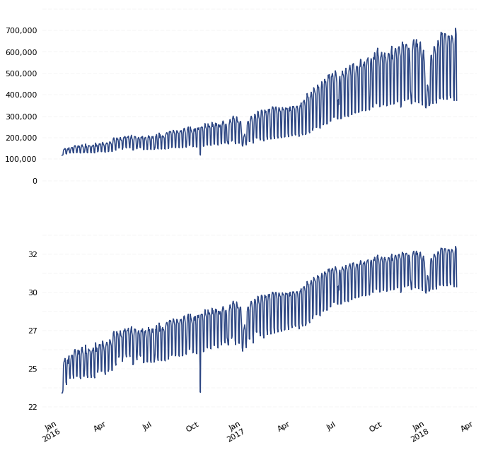
If we plot our newly transformed data alongside the untransformed data, we can see that the Box-Cox transformation was able to remove much of the increasing variance in our observations over time:
Forecasting
The first step in creating a forecast using Prophet is importing the fbprophet library into our R notebook:
library(prophet)
Once you've improted the prophet library, you're ready to fit a model to your historical data. You do this by calling the prophet() function using your prepared dataframe as an input:
m <- prophet(df)
Once you have used Prophet to fit the model using the Box-Cox transformed dataset, you can now start making predictions for future dates. Prophet has a built-in helper function make_future_dataframe to create a dataframe of future dates. The make_future_dataframe function lets you specify the frequency and number of periods you would like to forecast into the future. By default, the frequency is set to days. Since we are using daily periodicity data in this example, we will leave freq at it’s default and set the periods argument to 365, indicating that we would like to forecast 365 days into the future.
future <- make_future_dataframe(m, periods = 365)
We can now use the predict() function to make predictions for each row in the future dataframe.
forecast <- predict(m, future)
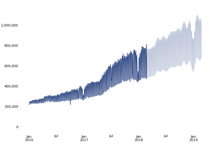
At this point, Prophet will have created a new dataframe assigned to the forecast variable that contains the forecasted values for future dates under a column called yhat, as well as uncertainty intervals and components for the forecast. We can visualize the forecast using Prophet’s built-in plot helper function:
plot(m, forecast)
In our example, our forecast looks as follows:
If you want to visualize the individual forecast components, you can use Prophet’s built-in plot_components function:
prophet_plot_components(m, forecast)
Running plot_components on our example data returns the following set of component visualizations:
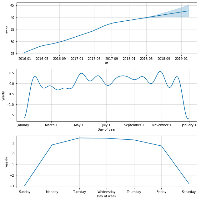
The forecast and component visualizations show that Prophet was able to accurately model the underlying trend in the data, while also accurately modeling weekly and yearly seasonality (e.g. lower order volume on weekend and holidays).
Inverse Box-Cox Transform
Since Prophet was used on the Box-Cox transformed data, you'll need to transform your forecasted values back to their original units. To transform your new forecasted values back to their original units, you will need to perform an inverse Box-Cox transform.
The R forecast library provides a built-in Inverse Box-Cox Transform function, called [InvBoxCox()](https://www.rdocumentation.org/packages/forecast/versions/8.1/topics/BoxCox). The InvBoxCox() function has two required inputs; a numeric vector or time series of class ts and and a lambda coefficient transformation parameter. We will inverse transform specific columns in our forecast dataframe, and supply the λ value we obtained earlier from our first Box-Cox transform stored in the lam variable:
inverse_forecast <- forecast
inverse_forecast <- column_to_rownames(inverse_forecast, var = "ds")
inverse_forecast$yhat_untransformed = InvBoxCox(forecast$yhat, lam)
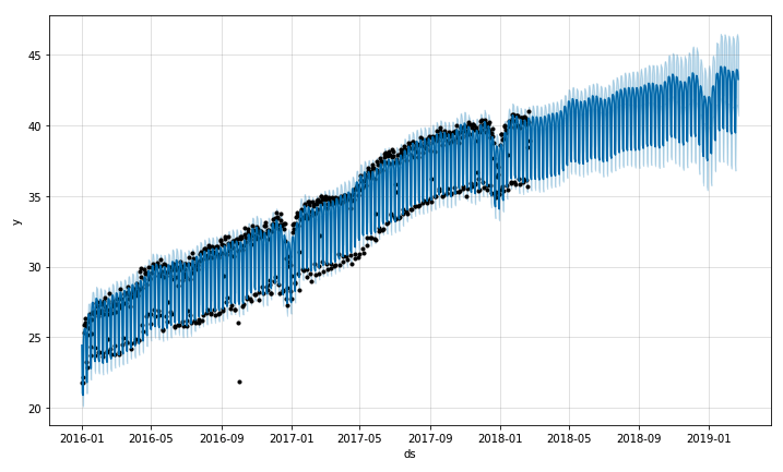
Now that your forecasted values are transformed back to their original units, you are able to visualize the forecasted values alongside the historical values: