
Python Tutorial
Learn Python for business analysis using real-world data. No coding experience necessary.
Start Now
Mode Studio
The Collaborative Data Science Platform
Pandas .groupby(), Lambda Functions, & Pivot Tables
Starting here? This lesson is part of a full-length tutorial in using Python for Data Analysis. Check out the beginning.
Goals of this lesson
In this lesson, you'll learn how to group, sort, and aggregate data to examine subsets and trends. Specifically, you’ll learn how to:
- Sample and sort data with
.sample(n=1)and.sort_values - Create Lambda functions
- Group data by columns with
.groupby() - Plot grouped data
- Group and aggregate data with
.pivot_tables()
Loading data into Mode Python notebooks
Mode is an analytics platform that brings together a SQL editor, Python notebook, and data visualization builder. Throughout this tutorial, you can use Mode for free to practice writing and running Python code.
For this lesson, you'll be using records of United States domestic flights from the US Department of Transportation. To access the data, you’ll need to use a bit of SQL. Here’s how:
- Log into Mode or create an account.
- Navigate to this report and click Duplicate. This will take you to the SQL Query Editor, with a query and results pre-populated.
- Click Python Notebook under Notebook in the left navigation panel. This will open a new notebook, with the results of the query loaded in as a dataframe.
- The first input cell is automatically populated with
datasets[0].head(n=5). Run this code so you can see the first five rows of the dataset.
datasets[0] is a list object. Nested inside this list is a DataFrame containing the results generated by the SQL query you wrote. To learn more about how to access SQL queries in Mode Python Notebooks, read this documentation.
Now you’re all ready to go.
About this data
In this lesson, you'll use records of United States domestic flights from the US Department of Transportation. It includes a record of each flight that took place from January 1-15 of 2015. Each record contains a number of values:
Flight Records
FlightDate	   Flight Date (yyyymmdd)
UniqueCarrier	Unique Carrier Code
FlightNum	    Flight Number (Flights on different days may have the same flight number)
Origin	       Origin Airport
Dest	         Destination Airport
DepDelay	     Difference in minutes between scheduled and actual departure time. Early departures show negative numbers.
ArrDelay	     Difference in minutes between scheduled and actual arrival time. Early arrivals show negative numbers.
Cancelled	    Cancelled Flight Indicator (1=Yes)
CarrierDelay	 Carrier Delay, in Minutes
WeatherDelay	 Weather Delay, in Minutes
NASDelay	     National Air System Delay, in Minutes
SecurityDelay	Security Delay, in Minutes
LateAircraftDelay	Late Aircraft Delay, in Minutes
Carrier Codes
AA	American Airlines Inc.
OO	SkyWest Airlines Inc.
DL	Delta Air Lines Inc.
NK	Spirit Air Lines
HA	Hawaiian Airlines Inc.
WN	Southwest Airlines Co.
B6	JetBlue Airways
US	US Airways Inc.
AS	Alaska Airlines Inc.
MQ	Envoy Air
F9	Frontier Airlines Inc.
VX	Virgin America
EV	ExpressJet Airlines Inc.
UA	United Air Lines Inc.
For more visual exploration of this dataset, check out this estimator of which flight will get you there the fastest on FiveThirtyEight.
Getting oriented with the data
After following the steps above, go to your notebook and import NumPy and Pandas, then assign your DataFrame to the data variable so it's easy to keep track of:
import pandas as pd
import numpy as np
data = datasets[0] # assign SQL query results to the data variable
data = data.fillna(np.nan)
Sampling and sorting data
.sample()
The .sample() method lets you get a random set of rows of a DataFrame. Set the parameter n= equal to the number of rows you want. Sampling the dataset is one way to efficiently explore what it contains, and can be especially helpful when the first few rows all look similar and you want to see diverse data.
Grab a sample of the flight data to preview what kind of data you have. Re-run this cell a few times to get a better idea of what you're seeing:
data.sample(n=5)
| flight_date | unique_carrier | flight_num | origin | dest | arr_delay | cancelled | distance | carrier_delay | weather_delay | late_aircraft_delay | nas_delay | security_delay | actual_elapsed_time | |
|---|---|---|---|---|---|---|---|---|---|---|---|---|---|---|
| 53014 | 2015-01-12 00:00:00 | DL | 1516.0 | DEN | ATL | -4.0 | 0.0 | 1199.0 | NaN | NaN | NaN | NaN | NaN | 179.0 |
| 106774 | 2015-01-13 00:00:00 | WN | 1613.0 | SLC | PHX | -15.0 | 0.0 | 507.0 | NaN | NaN | NaN | NaN | NaN | 88.0 |
| 191165 | 2015-01-04 00:00:00 | MQ | 3065.0 | GSO | DFW | NaN | 1.0 | 999.0 | NaN | NaN | NaN | NaN | NaN | NaN |
| 150360 | 2015-01-06 00:00:00 | US | 2062.0 | MCO | CLT | -16.0 | 0.0 | 468.0 | NaN | NaN | NaN | NaN | NaN | 85.0 |
| 168919 | 2015-01-05 00:00:00 | EV | 4724.0 | ORD | CAE | 77.0 | 0.0 | 667.0 | 77.0 | 0.0 | 0.0 | 0.0 | 0.0 | 103.0 |
.sort_values()
Now that you have a sense for what some random records look like, take a look at some of the records with the longest delays. This is likely a good place to start formulating hypotheses about what types of flights are typically delayed.
The values in the arr_delay column represent the number of minutes a given flight is delayed. Sort by that column in descending order to see the ten longest-delayed flights. Note that values of 0 indicate that the flight was on time:
data.sort_values(by='arr_delay', ascending=False)[:10]
| flight_date | unique_carrier | flight_num | origin | dest | arr_delay | cancelled | distance | carrier_delay | weather_delay | late_aircraft_delay | nas_delay | security_delay | actual_elapsed_time | |
|---|---|---|---|---|---|---|---|---|---|---|---|---|---|---|
| 11073 | 2015-01-11 00:00:00 | AA | 1595.0 | AUS | DFW | 1444.0 | 0.0 | 190.0 | 1444.0 | 0.0 | 0.0 | 0.0 | 0.0 | 59.0 |
| 10214 | 2015-01-13 00:00:00 | AA | 1487.0 | OMA | DFW | 1392.0 | 0.0 | 583.0 | 1392.0 | 0.0 | 0.0 | 0.0 | 0.0 | 117.0 |
| 12430 | 2015-01-03 00:00:00 | AA | 1677.0 | MEM | DFW | 1384.0 | 0.0 | 432.0 | 1380.0 | 0.0 | 0.0 | 4.0 | 0.0 | 104.0 |
| 8443 | 2015-01-04 00:00:00 | AA | 1279.0 | OMA | DFW | 1237.0 | 0.0 | 583.0 | 1222.0 | 0.0 | 15.0 | 0.0 | 0.0 | 102.0 |
| 10328 | 2015-01-05 00:00:00 | AA | 1495.0 | EGE | DFW | 1187.0 | 0.0 | 721.0 | 1019.0 | 0.0 | 168.0 | 0.0 | 0.0 | 127.0 |
| 36570 | 2015-01-04 00:00:00 | DL | 1435.0 | MIA | MSP | 1174.0 | 0.0 | 1501.0 | 1174.0 | 0.0 | 0.0 | 0.0 | 0.0 | 231.0 |
| 36495 | 2015-01-04 00:00:00 | DL | 1367.0 | ROC | ATL | 1138.0 | 0.0 | 749.0 | 1112.0 | 0.0 | 0.0 | 26.0 | 0.0 | 171.0 |
| 59072 | 2015-01-14 00:00:00 | DL | 1687.0 | SAN | MSP | 1084.0 | 0.0 | 1532.0 | 1070.0 | 0.0 | 0.0 | 14.0 | 0.0 | 240.0 |
| 32173 | 2015-01-05 00:00:00 | AA | 970.0 | LAS | LAX | 1042.0 | 0.0 | 236.0 | 1033.0 | 0.0 | 9.0 | 0.0 | 0.0 | 66.0 |
| 56488 | 2015-01-12 00:00:00 | DL | 2117.0 | ATL | COS | 1016.0 | 0.0 | 1184.0 | 1016.0 | 0.0 | 0.0 | 0.0 | 0.0 | 193.0 |
Wow. The longest delay was 1444 minutes—a whole day! The worst delays occurred on American Airlines flights to DFW (Dallas-Fort Worth), and they don't seem to have been delayed due to weather (you can tell because the values in the weather_delay column are 0).
Lambda functions
January can be a tough time for flying—snowstorms in New England and the Midwest delayed travel at the beginning of the month as people got back to work. But how often did delays occur from January 1st-15th?
To quickly answer this question, you can derive a new column from existing data using an in-line function, or a lambda function.
In the previous lesson, you created a column of boolean values (True or False) in order to filter the data in a DataFrame. Here, it makes sense to use the same technique to segment flights into two categories: delayed and not delayed.
The technique you learned in the previous lesson calls for you to create a function, then use the .apply() method like this:
def is_delayed(x):
    return x > 0
data['delayed'] = data['arr_delay'].apply(is_delayed)
For very short functions or functions that you do not intend to use multiple times, naming the function may not be necessary. The function used above could be written more quickly as a lambda function, or a function without a name.
The following code does the same thing as the above cell, but is written as a lambda function:
data['delayed'] = data['arr_delay'].apply(lambda x: x > 0)
Let's break it down:
lambda— this is a lambda functionx:— the parameter name within the functionx > 0— what to do with the parameter
Your biggest question might be, What is x? The .apply() method is going through every record one-by-one in the data['arr_delay'] series, where x is each record. Just as the def function does above, the lambda function checks if the value of each arr_delay record is greater than zero, then returns True or False.
This might be a strange pattern to see the first few times, but when you’re writing short functions, the lambda function allows you to work more quickly than the def function.
Calculating percentages
Now that you have determined whether or not each flight was delayed, you can get some information about the aggregate trends in flight delays.
Count the values in this new column to see what proportion of flights are delayed:
data['delayed'].value_counts()
False    103037
True      98627
Name: delayed, dtype: int64
The value_counts() method actually returns the two numbers, ordered from largest to smallest. You can use them to calculate the percentage of flights that were delayed:
not_delayed = data['delayed'].value_counts()[0] # first value of the result above
delayed = data['delayed'].value_counts()[1] # second value of the result above
total_flights = not_delayed + delayed # total count of flights
print float(delayed) / total_flights # converting to float to get a float result
0.48906597112
51% of flights had some delay. That's pretty high! Better bring extra movies.
Floats and integers
You might have noticed in the example above that we used the float() function. Try to answer the following question and you'll see why:
What is 4 divided by 3?
4/3
1
One? That's weird.
This calculation uses whole numbers, called integers. When you use arithmetic on integers, the result is a whole number without the remainder, or everything after the decimal. This can cause some confusing results if you don't know what to expect. Turn at least one of the integers into a float, or numbers with decimals, to get a result with decimals.
float(4)/3
1.3333333333333333
In Python, if at least one number in a calculation is a float, the outcome will be a float.
Besides being delayed, some flights were cancelled. Those flights had a delay of "0", because they never left. What percentage of the flights in this dataset were cancelled? A percentage, by definition, falls between 0 and 1, which means it's probably not an int.
data['cancelled'].value_counts() # count the (0, 1) values
0.0    196873
1.0      4791
Name: cancelled, dtype: int64
not_delayed, delayed = data['cancelled'].value_counts()
print delayed / (delayed + not_delayed), '<- without conversion'
print float(delayed) / (delayed + not_delayed), '<- _with_ conversion!'
0 <- without conversion
0.02375733894 <- _with_ conversion!
Across all flights, about 2.38% were cancelled.
Python will also infer that a number is a float if it contains a decimal, for example:
4.0/3
1.3333333333333333
Grouping data by categorical values
If half of the flights were delayed, were delays shorter or longer on some airlines as opposed to others? To compare delays across airlines, we need to group the records of airlines together. Boolean indexing won't work for this—it can only separate the data into two categories: one that is true, and one that is false (or, in this case, one that is delayed and one that is not delayed). What we need here is two categories (delayed and not delayed) for each airline.
.groupby()
The .groupby() function allows us to group records into buckets by categorical values, such as carrier, origin, and destination in this dataset.
Since you already have a column in your data for the unique_carrier, and you created a column to indicate whether a flight is delayed, you can simply pass those arguments into the groupby() function. This will create a segment for each unique combination of unique_carrier and delayed. In other words, it will create exactly the type of grouping described in the previous two paragraphs:
group_by_carrier = data.groupby(['unique_carrier','delayed'])
Think of groupby() as splitting the dataset data into buckets by carrier (‘unique_carrier’), and then splitting the records inside each carrier bucket into delayed or not delayed (‘delayed’). The result is assigned to the group_by_carrier variable.
What happens next gets tricky. If you just look at the group_by_carrier variable, you'll see that it is a DataFrameGroupBy object. You can think of that as instructions on how to group, but without instructions on how to display values:
group_by_carrier
<pandas.core.groupby.DataFrameGroupBy object at 0x10c6df610>
You need to provide instructions on what values to display. For example:
You're grouping all of the rows that share the same carrier, as well as all the rows that share the same value for delayed. You need to tell the function what to do with the other values. You could do any number of things:
- average the number of minutes of delay
- sum the total number of minutes of delay
You've already started down the path of simply determining the proportion of flights that are delayed or not, so you might as well finish the problem. Instead of averaging or summing, use .size() to count the number of rows in each grouping:
group_by_carrier.size()
unique_carrier  delayed
AA              False       8912
                True        9841
AS              False       3527
                True        2104
B6              False       4832
                True        4401
DL              False      17719
                True        9803
EV              False      10596
                True       11371
F9              False       1103
                True        1848
HA              False       1351
                True        1354
MQ              False       4692
                True        8060
NK              False       1550
                True        2133
OO              False       9977
                True       10804
UA              False       7885
                True        8624
US              False       7850
                True        6353
VX              False       1254
                True         781
WN              False      21789
                True       21150
dtype: int64
That's exactly what you're looking for! It's a little hard to read, though. Pandas has a handy .unstack() method—use it to convert the results into a more readable format and store that as a new variable, count_delays_by_carrier
count_delays_by_carrier = group_by_carrier.size().unstack()
count_delays_by_carrier
| delayed | False | True |
|---|---|---|
| unique_carrier | ||
| AA | 8912 | 9841 |
| AS | 3527 | 2104 |
| B6 | 4832 | 4401 |
| DL | 17719 | 9803 |
| EV | 10596 | 11371 |
| F9 | 1103 | 1848 |
| HA | 1351 | 1354 |
| MQ | 4692 | 8060 |
| NK | 1550 | 2133 |
| OO | 9977 | 10804 |
| UA | 7885 | 8624 |
| US | 7850 | 6353 |
| VX | 1254 | 781 |
| WN | 21789 | 21150 |
.groupby() is a tough but powerful concept to master, and a common one in analytics especially. For example, a marketing analyst looking at inbound website visits might want to group data by channel, separating out direct email, search, promotional content, advertising, referrals, organic visits, and other ways people found the site. The analyst might also want to examine retention rates among certain groups of people (known as cohorts) or how people who first visited the site around the same time behaved. Learn more about retention analysis among cohorts in this blog post.
See Wes McKinney's blog post on groupby for more examples and explanation.
SQL GROUP BY
This is very similar to the GROUP BY clause in SQL, but with one key difference:
Retain data after aggregating: By using .groupby(), we retain the original data after we've grouped everything. You can still access the original dataset using the data variable, but you can also access the grouped dataset using the new group_by_carrier. When using SQL, you cannot directly access both the grouped/aggregated dataset and the original dataset (technically you can, but it would not be straightforward).
Nevertheless, here’s how the above grouping would work in SQL, using COUNT, CASE, and GROUP BY:
SELECT unique_carrier,
    COUNT(CASE WHEN arr_delay <= 0 OR arr_delay IS NULL THEN 'not_delayed' END) AS not_delayed,
    COUNT(CASE WHEN arr_delay > 0 THEN 'delayed' END) AS delayed
  FROM tutorial.us_flights
    GROUP BY unique_carrier
For more on how the components of this query, see the SQL lessons on CASE statements and GROUP BY.
Plotting grouped data
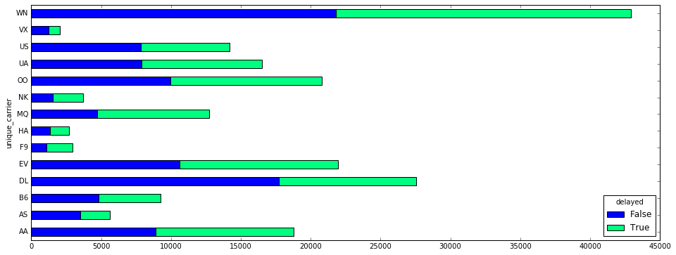
Though Southwest (WN) had more delays than any other airline, all the airlines had proportionally similar rates of delayed flights. You can see this by plotting the delayed and non-delayed flights.
Use a new parameter in .plot() to stack the values vertically (instead of allowing them to overlap) called stacked=True:
count_delays_by_carrier.plot(kind='barh', stacked=True, figsize=[16,6], colormap='winter')
If you need a refresher on making bar charts with Pandas, check out this earlier lesson.
Customizing plots with .plot() parameters
You can customize plots a number of ways. Here's a quick guide to common parameters:
kind=: 'line', 'bar', 'barh', 'hist', 'box', 'area', 'scatter'figsize=: (width, height) in inchescolormap=: a long list of color palettes, including: 'autumn', 'winter', 'summer'title=: a stringstacked=: stack the values vertically (instead of allowing them to overlap)
Here's the full list of plot parameters for DataFrames.
Practice Problem
How many flights were delayed longer than 20 minutes?
Bonus Question: What proportion of delayed flights does this represent?
View SolutionPivot tables
A pivot table is composed of counts, sums, or other aggregations derived from a table of data. You may have used this feature in spreadsheets, where you would choose the rows and columns to aggregate on, and the values for those rows and columns. It allows us to summarize data as grouped by different values, including values in categorical columns.
You can define how values are grouped by:
index=("Rows" in Excel)columns=
We define which values are summarized by:
values=the name of the column of values to be aggregated in the ultimate table, then grouped by the Index and Columns and aggregated according to the Aggregation Function
We define how values are summarized by:
aggfunc=(Aggregation Function) how rows are summarized, such assum,mean, orcount
Let's create a .pivot_table() of the number of flights each carrier flew on each day:
flights_by_carrier = data.pivot_table(index='flight_date', columns='unique_carrier', values='flight_num', aggfunc='count')
flights_by_carrier.head()
| unique_carrier | AA | AS | B6 | DL | EV | F9 | HA | MQ | NK | OO | UA | US | VX | WN |
|---|---|---|---|---|---|---|---|---|---|---|---|---|---|---|
| flight_date | ||||||||||||||
| 2015-01-02 | 1545 | 477 | 759 | 2271 | 1824 | 254 | 224 | 1046 | 287 | 1763 | 1420 | 1177 | 176 | 3518 |
| 2015-01-03 | 1453 | 449 | 711 | 2031 | 1744 | 192 | 202 | 937 | 285 | 1681 | 1233 | 1028 | 160 | 3328 |
| 2015-01-04 | 1534 | 458 | 759 | 2258 | 1833 | 249 | 206 | 1027 | 284 | 1731 | 1283 | 1158 | 169 | 3403 |
| 2015-01-05 | 1532 | 433 | 754 | 2212 | 1811 | 264 | 209 | 1039 | 288 | 1737 | 1432 | 1157 | 174 | 3506 |
| 2015-01-06 | 1400 | 415 | 692 | 2054 | 1686 | 249 | 202 | 966 | 279 | 1527 | 1294 | 1003 | 152 | 3396 |
In this table, you can see the count of flights (flight_num) flown by each unique_carrier on each flight_date. This is extremely powerful, because you don't have to write a separate function for each carrier—this one function handles counts for all of them.
.pivot_table() does not necessarily need all four arguments, because it has some smart defaults. If we pivot on one column, it will default to using all other numeric columns as the index (rows) and take the average of the values. For example, if we want to pivot and summarize on flight_date:
data.pivot_table(columns='flight_date')
| flight_date | 2015-01-02 | 2015-01-03 | 2015-01-04 | 2015-01-05 | 2015-01-06 | 2015-01-07 | 2015-01-08 | 2015-01-09 | 2015-01-10 | 2015-01-11 | 2015-01-12 | 2015-01-13 | 2015-01-14 |
|---|---|---|---|---|---|---|---|---|---|---|---|---|---|
| actual_elapsed_time | 141.688442 | 145.950033 | 145.111664 | 140.607814 | 137.699987 | 136.297427 | 138.249851 | 137.045859 | 137.876833 | 138.712463 | 139.096045 | 134.649796 | 133.110117 |
| arr_delay | 9.838904 | 25.461860 | 31.975011 | 18.811310 | 21.299274 | 11.955429 | 13.316482 | 12.255611 | 1.922475 | 10.187042 | 18.563998 | 3.162599 | -0.817102 |
| cancelled | 0.015352 | 0.021446 | 0.026480 | 0.026287 | 0.025792 | 0.019459 | 0.050784 | 0.029298 | 0.015392 | 0.023993 | 0.027442 | 0.012978 | 0.011469 |
| carrier_delay | 16.668783 | 18.023806 | 18.213584 | 17.986333 | 16.751224 | 15.317566 | 19.767890 | 18.768564 | 25.002997 | 17.142741 | 15.063235 | 18.112939 | 22.049189 |
| delayed | 0.500209 | 0.648050 | 0.679244 | 0.548707 | 0.544695 | 0.483912 | 0.419639 | 0.468328 | 0.345917 | 0.436424 | 0.551360 | 0.382279 | 0.302835 |
| distance | 839.785915 | 848.749320 | 838.077666 | 820.224801 | 784.111329 | 785.939182 | 792.963770 | 793.554910 | 830.779650 | 809.407279 | 791.471614 | 779.262121 | 782.294072 |
| flight_num | 2284.698047 | 2287.225541 | 2268.050514 | 2233.375030 | 2238.016324 | 2237.701561 | 2238.148479 | 2237.685657 | 2484.358312 | 2271.538701 | 2246.031407 | 2249.280171 | 2241.273711 |
| late_aircraft_delay | 21.317207 | 26.525643 | 31.864547 | 26.294995 | 28.462557 | 22.112744 | 26.855823 | 26.280862 | 17.287712 | 26.642197 | 25.970956 | 19.288743 | 18.260073 |
| nas_delay | 9.005254 | 13.782660 | 15.452955 | 14.294107 | 17.223935 | 14.835132 | 18.485873 | 11.877020 | 6.972028 | 12.194943 | 16.471140 | 11.319079 | 9.395081 |
| security_delay | 0.056480 | 0.139603 | 0.048513 | 0.034966 | 0.067452 | 0.037887 | 0.134671 | 0.042633 | 0.057942 | 0.044589 | 0.010294 | 0.043129 | 0.090529 |
| weather_delay | 1.610552 | 2.094342 | 2.142729 | 3.627618 | 4.768631 | 4.078760 | 8.717983 | 3.531506 | 2.838661 | 3.487765 | 3.433456 | 1.489035 | 3.231816 |
In the table above, we get the average of values by day, across all numberic columns. That was quick!
Reasonable delays
Several columns in the dataset indicate the reasons for the flight delay. You now know that about half of flights had delays—what were the most common reasons? Was there a lot of snow in January? Did the planes freeze up?
To find out, you can pivot on the date and type of delay, delays_list, summing the number of minutes of each type of delay:
delays_list = ['carrier_delay','weather_delay','late_aircraft_delay','nas_delay','security_delay']
flight_delays_by_day = data.pivot_table(index='flight_date', values=delays_list, aggfunc='sum')
flight_delays_by_day
| carrier_delay | late_aircraft_delay | nas_delay | security_delay | weather_delay | |
|---|---|---|---|---|---|
| flight_date | |||||
| 2015-01-02 | 76143.0 | 97377.0 | 41136.0 | 258.0 | 7357.0 |
| 2015-01-03 | 122652.0 | 180507.0 | 93791.0 | 950.0 | 14252.0 |
| 2015-01-04 | 142667.0 | 249595.0 | 121043.0 | 380.0 | 16784.0 |
| 2015-01-05 | 101335.0 | 148146.0 | 80533.0 | 197.0 | 20438.0 |
| 2015-01-06 | 92383.0 | 156971.0 | 94990.0 | 372.0 | 26299.0 |
| 2015-01-07 | 66708.0 | 96301.0 | 64607.0 | 165.0 | 17763.0 |
| 2015-01-08 | 74861.0 | 101703.0 | 70006.0 | 510.0 | 33015.0 |
| 2015-01-09 | 80123.0 | 112193.0 | 50703.0 | 182.0 | 15076.0 |
| 2015-01-10 | 50056.0 | 34610.0 | 13958.0 | 116.0 | 5683.0 |
| 2015-01-11 | 63051.0 | 97990.0 | 44853.0 | 164.0 | 12828.0 |
| 2015-01-12 | 81944.0 | 141282.0 | 89603.0 | 56.0 | 18678.0 |
| 2015-01-13 | 49557.0 | 52774.0 | 30969.0 | 118.0 | 4074.0 |
| 2015-01-14 | 42136.0 | 34895.0 | 17954.0 | 173.0 | 6176.0 |
The results in this table are the sum of minutes delayed, by type of delay, by day. How do each of the flight delays contribute to overall delay each day?
Let's build an area chart, or a stacked accumulation of counts, to illustrate the relative contribution of the delays. You can pass the arguments kind='area' and stacked=True to create the stacked area chart, colormap='autumn' to give it vibrant color, and figsize=[16,6] to make it bigger:
flight_delays_by_day.plot(kind='area', figsize=[16,6], stacked=True, colormap='autumn') # area plot
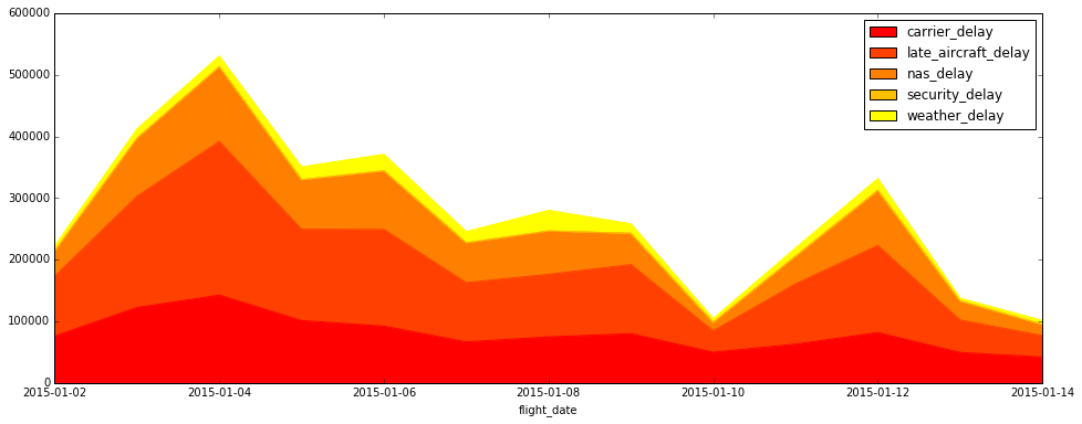
It looks like late aircraft caused a large number of the delays on the 4th and the 12th of January. One hypothesis is that snow kept planes grounded and unable to continue their routes. In the next lesson, we'll dig into which airports contributed most heavily to delays.
Practice Problem
Which airlines contributed most to the sum total minutes of delay? Pivot the daily sum of delay minutes by airline.
Bonus Points: Plot the delays as a stacked bar chart.
View Solution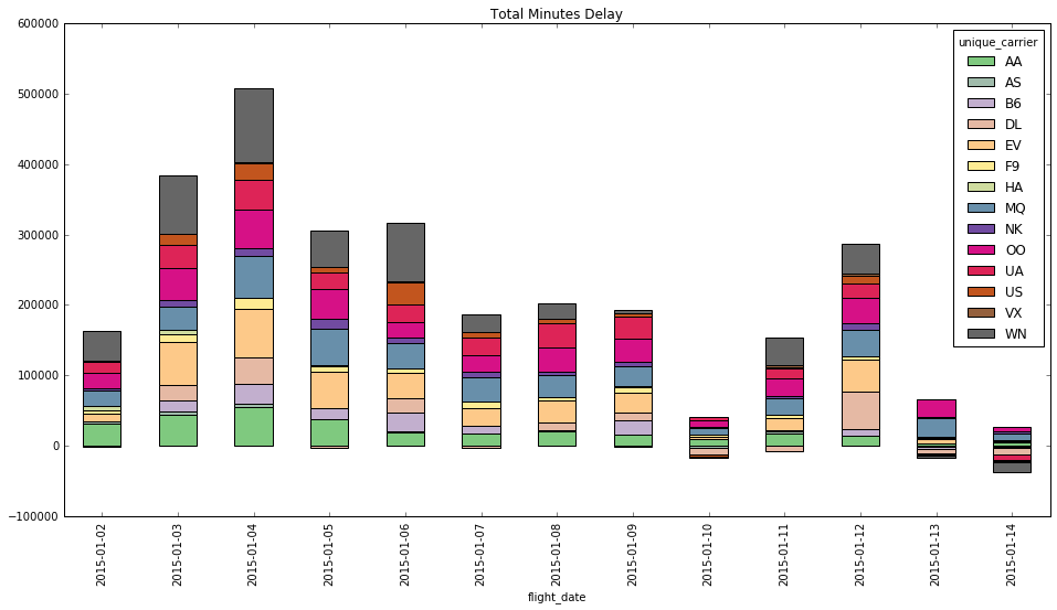
Lesson summary:
That was a ton of new material! In this Python lesson, you learned about:
- Sampling and sorting data with
.sample(n=1)and.sort_values - Lambda functions
- Grouping data by columns with
.groupby() - Plotting grouped data
- Grouping and aggregate data with
.pivot_tables()
In the next lesson, you'll learn about data distributions, binning, and box plots.
Next Lesson
Python Histograms, Box Plots, & Distributions