Performance Tuning SQL Queries

Starting here? This lesson is part of a full-length tutorial in using SQL for Data Analysis. Check out the beginning.

In this lesson we'll cover:

• The theory behind query run time
• Reducing table size
• Making joins less complicated
• EXPLAIN

What is SQL Performance Tuning?

SQL tuning is the process of improving SQL queries to accelerate your servers performance. It's general purpose is to reduce the amount of time it takes a user to receive a result after issuing a query, and to reduce the amount of resources used to process a query. The lesson on subqueries introduced the idea that you can sometimes create the same desired result set with a faster-running query. In this lesson, you'll learn to identify when your queries can be improved, and how to improve them.

The theory behind query run time

A database is a piece of software that runs on a computer, and is subject to the same limitations as all software—it can only process as much information as its hardware is capable of handling. The way to make a query run faster is to reduce the number of calculations that the software (and therefore hardware) must perform. To do this, you'll need some understanding of how SQL actually makes calculations. First, let's address some of the high-level things that will affect the number of calculations you need to make, and therefore your querys runtime:

• Table size: If your query hits one or more tables with millions of rows or more, it could affect performance.
• Joins: If your query joins two tables in a way that substantially increases the row count of the result set, your query is likely to be slow. There's an example of this in the subqueries lesson.
• Aggregations: Combining multiple rows to produce a result requires more computation than simply retrieving those rows.

Query runtime is also dependent on some things that you can't really control related to the database itself:

• Other users running queries: The more queries running concurrently on a database, the more the database must process at a given time and the slower everything will run. It can be especially bad if others are running particularly resource-intensive queries that fulfill some of the above criteria.
• Database software and optimization: This is something you probably can't control, but if you know the system you're using, you can work within its bounds to make your queries more efficient.

For now, let's ignore the things you can't control and work on the things you can.

Reducing table size

Filtering the data to include only the observations you need can dramatically improve query speed. How you do this will depend entirely on the problem you're trying to solve. For example, if you've got time series data, limiting to a small time window can make your queries run much more quickly:

SELECT *
  FROM benn.sample_event_table
 WHERE event_date >= '2014-03-01'
   AND event_date <  '2014-04-01'

Keep in mind that you can always perform exploratory analysis on a subset of data, refine your work into a final query, then remove the limitation and run your work across the entire dataset. The final query might take a long time to run, but at least you can run the intermediate steps quickly.

This is why Mode enforces a LIMIT clause by default—100 rows is often more than you need to determine the next step in your analysis, and it's a small enough dataset that it will return quickly.

It's worth noting that LIMIT doesn't quite work the same way with aggregations—the aggregation is performed, then the results are limited to the specified number of rows. So if you're aggregating into one row as below, LIMIT 100 will do nothing to speed up your query:

SELECT COUNT(*)
  FROM benn.sample_event_table
 LIMIT 100

If you want to limit the dataset before performing the count (to speed things up), try doing it in a subquery:

SELECT COUNT(*)
  FROM (
    SELECT *
      FROM benn.sample_event_table
     LIMIT 100
       ) sub

Note: Using LIMIT this will dramatically alter your results, so you should use it to test query logic, but not to get actual results.

In general, when working with subqueries, you should make sure to limit the amount of data you're working with in the place where it will be executed first. This means putting the LIMIT in the subquery, not the outer query. Again, this is for making the query run fast so that you can test—NOT for producing good results.

Making joins less complicated

In a way, this is an extension of the previous tip. In the same way that it's better to reduce data at a point in the query that is executed early, it's better to reduce table sizes before joining them. Take this example, which joins information about college sports teams onto a list of players at various colleges:

SELECT teams.conference AS conference,
       players.school_name,
       COUNT(1) AS players
  FROM benn.college_football_players players
  JOIN benn.college_football_teams teams
    ON teams.school_name = players.school_name
 GROUP BY 1,2

There are 26,298 rows in benn.college_football_players. That means that 26,298 rows need to be evaluated for matches in the other table. But if the benn.college_football_players table was pre-aggregated, you could reduce the number of rows that need to be evaluated in the join. First, let's look at the aggregation:

SELECT players.school_name,
       COUNT(*) AS players
  FROM benn.college_football_players players
 GROUP BY 1

The above query returns 252 results. So dropping that in a subquery and then joining to it in the outer query will reduce the cost of the join substantially:

SELECT teams.conference,
       sub.*
  FROM (
        SELECT players.school_name,
               COUNT(*) AS players
          FROM benn.college_football_players players
         GROUP BY 1
       ) sub
  JOIN benn.college_football_teams teams
  ON teams.school_name = sub.school_name

In this particular case, you won't notice a huge difference because 30,000 rows isn't too hard for the database to process. But if you were talking about hundreds of thousands of rows or more, you'd see a noticeable improvement by aggregating before joining. When you do this, make sure that what you're doing is logically consistent—you should worry about the accuracy of your work before worrying about run speed.

EXPLAIN

You can add EXPLAIN at the beginning of any (working) query to get a sense of how long it will take. It's not perfectly accurate, but it's a useful tool. Try running this:

EXPLAIN
SELECT *
  FROM benn.sample_event_table
 WHERE event_date >= '2014-03-01'
   AND event_date < '2014-04-01'
 LIMIT 100

You'll get this output. It's called the Query Plan, and it shows the order in which your query will be executed:

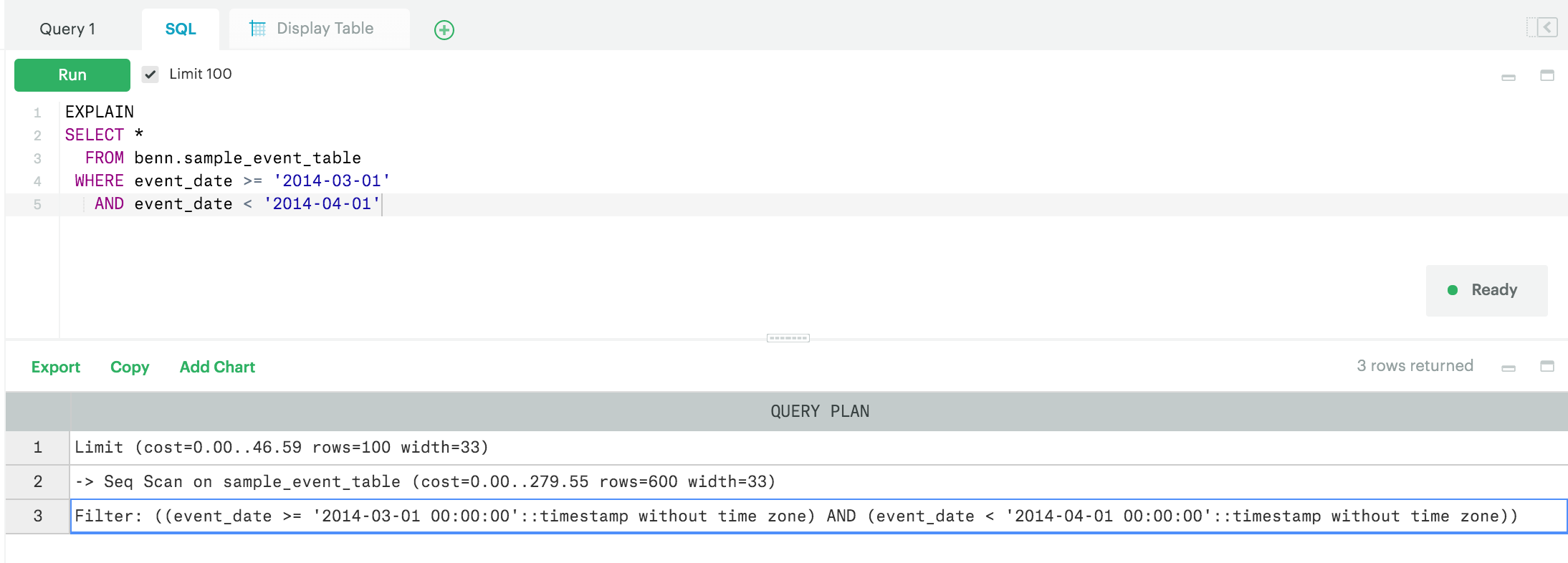
The entry at the bottom of the list is executed first. So this shows that the WHERE clause, which limits the date range, will be executed first. Then, the database will scan 600 rows (this is an approximate number). You can see the cost listed next to the number of rows—higher numbers mean longer run time. You should use this more as a reference than as an absolute measure. To clarify, this is most useful if you run EXPLAIN on a query, modify the steps that are expensive, then run EXPLAIN again to see if the cost is reduced. Finally, the LIMIT clause is executed last and is really cheap to run (24.65 vs 147.87 for the WHERE clause).

For more detail, check out the Postgres Documentation.