The Top 5 Most Popular Window Functions and How to Use Them

Nate Coleman, Data Scientist
July 23, 2020
NaN minute read

The data team at Mode loves SQL. We code it, write about it, and empower people to use it all over the world. So, in that vein, we thought it would be fun to use some SQL to analyze some SQL! That said, we don’t believe in analysis for the sake of analysis, so we did some research to help our readers better understand one of the most powerful tools in SQL—window functions.
What is a window function?
We’re going to borrow PostgreSQL’s definition:
"A window function performs a calculation across a set of table rows that are somehow related to the current row. This is comparable to the type of calculation that can be done with an aggregate function. But unlike regular aggregate functions, use of a window function does not cause rows to become grouped into a single output row — the rows retain their separate identities. Behind the scenes, the window function is able to access more than just the current row of the query result."
For those not familiar with the concept of window functions, I recommend you take a look at the Mode tutorial on this subject before moving on.
Okay, so we were curious to understand which window functions are most commonly used, so we built a window (pun intended) into our customer’s usage of these types of calculations.
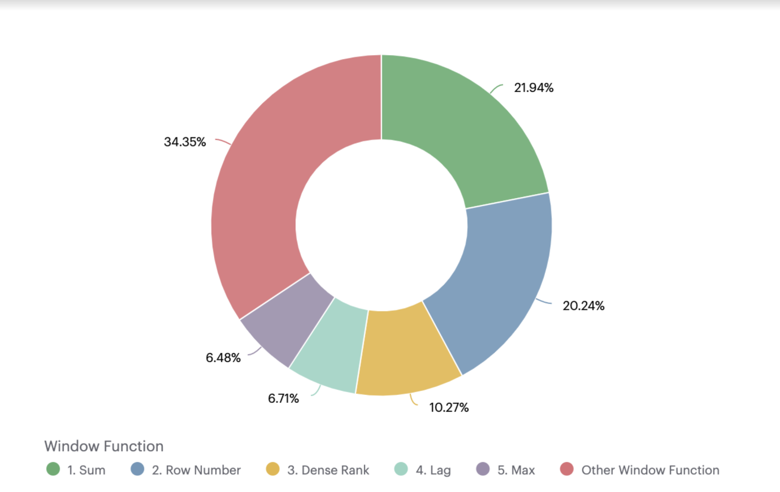
We built a dataset of all queries created since January 1, 2019 and used some regex magic to extract window functions. Then we counted up uses of each window function in our dataset and identified the most frequently used. The chart below shows the percent of all window function use attributed to the top five most used.

Given that these are the most frequently used window functions, we thought it would be useful to provide examples of how to use them—both for folks who are new to SQL, and for SQL users like me, who, sometimes forget a little syntax.
1. Sum
One of the most common use cases for the SUM window function is calculating a running sum. Let’s look at an example:
SELECT o.occurred_at,
       SUM(o.gloss_qty) OVER(ORDER BY o.occurred_at) as running_gloss_orders
  FROM demo.orders o
To break down the syntax here, SUM(o.gloss_qty) defines the aggregation—we’re going to be taking a sum of gloss_qty. Next, the OVER(ORDER BY o.occurred_at) clause tells your SQL engine to go row-by-row and take the sum of every record of gloss_qty in order by occurred_at up until the row it’s currently looking at.
We can also create separate running sums for different groups within our dataset by adding a PARTITION BY as seen below:
SELECT o.occurred_at,
	     o.account_id,
	     SUM(o.gloss_qty) OVER(PARTITION BY o.account_id
                          ORDER BY o.occurred_at) as running_gloss_orders
  FROM demo.orders o
2. Row Number
Ah, row number. This is my favorite window function. I commonly use ROW_NUMBER when I want to return the most recent record of a table I’m working with. ROW_NUMBER simply returns the number of the given row starting with 1, which is the first record as defined by the ORDER BY. No need to specify a variable in the parenthesis here!
  WITH
	order_ranks as (
	   SELECT o.id,
	          o.account_id,
	          o.gloss_qty,
	          o.gloss_amt_usd,
	          ROW_NUMBER() OVER(PARTITION BY o.account_id
                           ORDER BY o.occurred_at DESC) as acct_order_rank
      FROM demo.orders o
)
	SELECT *
	 FROM  order_ranks
    WHERE  acct_order_rank = 1
Note the DESC in the ORDER BY —this tells the SQL engine to order rows by occurred_at in descending order (i.e. latest record first.) The query above returns the most recent record in the orders table for each account. This query also makes use of CTEs (if those are a foreign concept, read our latest post on them).
3. Dense Rank
DENSE_RANK works similar to ROW_NUMBER but differs in how it handles cases where two rows for the field specified in your ORDER BY have identical values. DENSE_RANK will assign rows with identical ORDER_BY values the same number, whereas ROW_NUMBER will produce distinct values.
    SELECT o.id,
	     o.account_id,
	     DATE_TRUNC('day',o.occurred_at) as occurred_day,
	     o.gloss_qty,
	     o.gloss_amt_usd,
	     DENSE_RANK() OVER(PARTITION BY o.account_id
                      ORDER BY DATE_TRUNC('day',o.occurred_at)) as dense_rank
    FROM demo.orders o
You can see in the results below that the 2nd and 3rd rows have the same dense_rank value of 2. Oh, and you’ll notice that the window function above uses a value derived from another SQL function DATE_TRUNC —nesting SQL functions inside a window function is fair game.

4. Lag
The LAG function is a favorite among time series junkies. This function allows you to compare a row to any of the rows preceding it. So for instance, if you wanted to find out how one order of gloss_qty compared to the previous orders, this is the function to use.
      SELECT o.id,
            o.occurred_at,
	        o.gloss_qty,
	        LAG(gloss_qty,1) OVER(ORDER BY o.occurred_at) as order_lag_1,
	        LAG(gloss_qty,2) OVER(ORDER BY o.occurred_at) as order_lag_2,
	        LAG(gloss_qty,3) OVER(ORDER BY o.occurred_at) as order_lag_3
     FROM   demo.orders o
Keep in mind that the first n rows of your data will be NULL (where n is the number of “lags” you specify). You can see this in the results of our query:

5. Max
And finally, we can top off this list with MAX. MAX works in the same way as SUM so I’m going to spice up the example with some more advanced syntax. Let’s say that I want to see how a current order stacks up against the highest order quantity among the previous 5 orders for gloss_qty. We can do this by adding in some additional syntax in our ORDER BY clause.
   SELECT o.id,
          o.occurred_at,
          o.gloss_qty,
          MAX(gloss_qty) OVER(ORDER BY o.occurred_at
                         ROWS BETWEEN 5 PRECEDING AND 1 PRECEDING) as max_order
FROM demo.orders o
After we specify the field to order by, we add a definition for our window size: ROWS BETWEEN 5 PRECEDING AND 1 PRECEDING. This clause is essentially saying, "look back across the previous 5 orders (not including the current order) and take the maximum value."
This syntax is flexible and can define any window across your dataset. The syntax typically looks like:
ORDER BY [order_var] ROWS BETWEEN window_start AND window_endwhere window_start and window_end take on one of the following values:
UNBOUNDED PRECEDING(i.e. all rows before the current row)[VALUE] PRECEDING(where [VALUE] = # of rows behind the current row to consider)CURRENT ROW[VALUE] FOLLOWING(where [VALUE] = # of rows ahead of the current row to consider)UNBOUNDED FOLLOWING(i.e. all rows after the current row)
Window functions are incredibly powerful tools that enable quick and flexible analysis, all in the context of the SQL editor. Now, go find your favorite window function and analyze away!

Watch a product tour of Mode
Curious about how Mode works? Sit back and watch the video—no reps ;)
Get our weekly data newsletter
Work-related distractions for data enthusiasts.


